It is a rite of passage for every algorithmic trader. You design a strategy, run a historical simulation over five years of market data, and the results are spectacular—a high Sharpe ratio, minimal drawdowns, and a smooth equity curve. Enthusiastic, you deploy the strategy to a live trading account. Weeks later, the real-world performance is stagnant, or worse, deeply in the red.
Why do backtest results almost always look better than live trading signals?
The discrepancy isn’t usually a flaw in your core trading thesis. Instead, it is driven by a series of structural, mathematical, and environmental asymmetries between the sterile world of historical data frames and the chaotic reality of live execution matching engines.
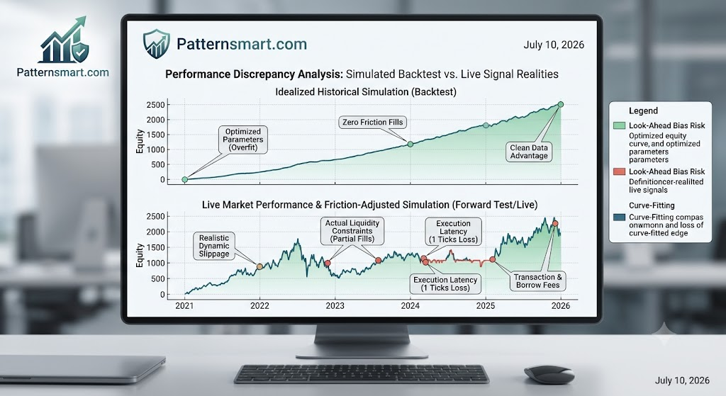
1. Structural Microstructure Asymmetries
A backtester typically operates under idealized market conditions. It assumes that if a price occurred historically, your order would have filled perfectly at that exact quote. Live markets do not work this way.
Slip-and-Fill Realities (The Execution Penalty)
In a backtest, buying at the “Close” of a 15-minute bar fills your position exactly at that printed price. In live trading, executing a market order at the close of a bar means your order must travel to the exchange, enter the order book, and match against available liquidity.
By the time your order processes, the market may have moved against you by a fraction of a percent. This discrepancy is known as slippage. While a loss of 0.05% per trade due to slippage sounds negligible, a high-frequency or day-trading strategy compounding this penalty over hundreds of trades will see its backtested edge completely erased.
The Order Book Illusion
Most basic backtesters assume infinite liquidity. If the historical data shows a low price of $150.00$, the backtester assumes you could have bought 10,000 shares at $150.00$.
Historical Data Point: Low = $150.00 (Volume = 200 shares)
Your Backtest Order: Buy 5,000 shares @ $150.00 -> SUCCESS (Illusion)

Live Market Reality:
Level 1 Liquidity: 200 shares @ $150.00
Level 2 Liquidity: 1,800 shares @ $150.05
Level 3 Liquidity: 3,000 shares @ $151.20
Your Actual Average Fill Price: $150.74 (Slippage Devastation)
In live environments, large orders sweep through the order book, driving your average fill price significantly higher (for longs) or lower (for shorts) than the asset’s printed baseline price.
2. Mathematical Optimization Traps
Sometimes the fault lies not within the market structure, but within how the strategy itself was formulated.
Overfitting and Curve Fitting
When developing a strategy, it is tempting to tweak parameters to find the “perfect” configuration (e.g., changing an RSI period from 14 to 11, or a MACD fast line from 12 to 9) because it yields a prettier historical equity curve.
This is known as curve fitting. You are no longer building a model that detects a recurring structural market anomaly; instead, you are simply coding an algorithm that memorizes the historical noise of a specific dataset. Because that exact sequence of noise will never happen again, the strategy fails immediately upon live deployment.
Survivorship and Selection Bias
If you backtest a stock trading strategy today using the current components of the S&P 500, your backtest suffers from survivorship bias. You are testing your strategy only on the companies that grew large and successful enough to be in the index in 2026. Your backtest completely ignores the hundreds of companies that went bankrupt, merged, or were delisted over the last decade.
3. Asymmetric Information: The Invisible Leak
The technical implementation of your code can create hidden informational advantages in a backtest that are physically impossible to replicate live.
| Optimization Vector | Backtest Environment | Live Trading Environment |
| Data Cleanliness | Corporate actions (splits, dividends) are perfectly back-adjusted. Bad ticks are scrubbed. | Raw data feeds include fragments, delayed quotes, unadjusted corporate actions, and temporary network drops. |
| Order Queue Status | Limit orders are assumed to fill immediately when the price touches the limit level. | Your limit order sits at the back of the exchange queue. The price can touch your limit and reverse without ever filling your order. |
| Transaction Friction | Static commission assumptions (e.g., flat $1.00 per trade). | Dynamic fees, exchange routing fees, borrow fees for shorting, and local financial transaction taxes. |
4. Engineering a Bulletproof Backtest
To force your historical simulations to reflect the harsh realities of live trading, you must transition from native backtesting to Defensive Backtesting Frameworks.
1.Enforce Strict Friction Latency Metrics:Phase 1.
Never run a backtest with zero friction. Artificially penalize every trade in your backtester by adding a conservative friction buffer (e.g., adding 1-2 ticks of slippage per trade plus the maximum possible broker fee tier). If your strategy cannot survive this penalty, it will not survive live trading.
2.Implement Out-of-Sample (OOS) Cross-Validation:Phase 2.
Divide your historical data into an “In-Sample” set (70%) and an “Out-of-Sample” set (30%). Build, tweak, and optimize your indicator parameters exclusively on the In-Sample data. Once finalized, lock the code and run it exactly once on the Out-of-Sample data. The OOS performance is the only true indicator of real-world viability.
3.Model Conservative Limit Order Fills:Phase 3.
Configure your backtester’s execution engine to only fill a limit order if the market price completely clears or breaches the target price by at least one full tick. If a limit buy is set at $100.00$, do not grant a fill if the bar’s low is exactly $100.00$. Require a low of $99.99$ or below to simulate moving to the front of the order queue.
5. The Sanity Check: Incubation
The ultimate defense against backtest deception is a mandatory incubation period.
Before allocating significant capital to a newly backtested strategy, deploy it to a forward-testing sandbox (paper trading or minimum-lot live execution) for a statistically significant period—typically 100 to 300 trades or 1-3 months depending on frequency.
Measure the mathematical variance between your simulated historical returns and your forward-tested incubation returns. If the live signals deviate significantly from the backtest boundaries, take the system offline: you haven’t found an alpha generator, you’ve simply found an uncompensated microstructural leak.
Contact us if you are looking for Professional Custom Trading Software Development Services